Phased Array Antenna Patterns – Part 2: Grating Lobes and Beam Squint

Peter Delos, Technical Lead, Bob Broughton, Director of Engineering and Jon Kraft, Senior Staff Field Applications Engineer, all with Analog Devices

Introduction

This is the second article of our three-part series on phased array antenna patterns. In Part 1, we introduced the phased array steering concept and looked at the influencers on array gain. In Part 2, we’ll discuss grating lobes and beam squint. Grating lobes can be hard to visualise, so we’ll draw on their similarity with signal aliasing in digital converters, then use that to think of a grating lobe as a spatial alias. Next, we explore the issue of beam squint. Beam squint is an un-focusing of the antenna across frequency when we use phase shift, instead of a true time delay, to steer the beam. We’ll also discuss the trade-off between these two steering methods and understand the impact of beam squint on typical systems.

An Introduction to Grating Lobes

So far, we have only seen the case where the element spacing is d = λ/2. Figure 1 begins to illustrate why an element spacing of λ/2 is such a common metric in phased arrays. Two cases are shown. First, in blue, the same 30° plot from Figure 11 in Part 1 is repeated. Next, the d/λ spacing is increased to 0.7 to show how the antenna pattern changes. With this increase in spacing, note how the beamwidth reduces, which is a positiveresult. The decreased spacing of nulls brings them closer together, which is also an acceptable result. But now there is a second angle, in this caseat –70°, where there is full array gain. This is a most unfortunate result. This replica of antenna gain is defined as a grating lobe and can be considered spatial aliasing.

Figure 1. Normalised array factor of a 32-element linear array at two different d/λ spacings.

Analogy to Sampled Systems

An analogy to visualise grating lobes is to think of aliasing in a sampled system. In an analogue-to-digital converter (ADC), under-sampling is oftenused when frequency planning a receiver architecture. Under-sampling involves purposefully reducing the sample rate (fS) such that the samplingprocess translates frequencies above fS/2 (the higher Nyquist zones) to appear as aliases in the first Nyquist zone. This causes those higherfrequencies to appear as if they were at a lower frequency at the output of the ADC.

A similar analogy can be considered in phased arrays, where the elements spatially sample the wavefront. The Nyquist theorem can be extended tothe spatial domain if we suggest that two samples - that is, elements - per wavelength are required to avoid aliasing. Therefore, if the elementspacing is greater than λ/2, we can consider this spatial aliasing.

Calculating Where Grating Lobes Appear

But where will these spatial aliases (grating lobes) appear? In Part 1, we showed the phase shift applied to the elements across the array as a function of beam angle.

Inversely, we can compute the beam angle as a function of phase shift.

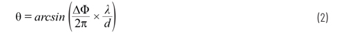
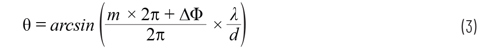
The arcsin function only produces real solutions for arguments between –1 and +1. Outside of these bounds, the solution is not real - the familiar“#NUM!” in spreadsheet software. Also note that the phase in Equation 2 is periodic and repeats every 2π. So, we could replace ∆Φ with (m × 2π + ∆Φ) in the beam steering equation to give Equation 3.

To avoid grating lobes, our goal is to obtain a single real solution. Mathematically, this is accomplished by keeping

If we do so, then all the spatial images (that is, m = ±1, ±2, etc.) will produce non-real arcsin results, and we can ignore them. But if we can’t do this,and therefore some values of m >0 produce real arcsin results, then we end up with multiple solutions: grating lobes.

Figure 2. The arcsin function application to grating lobes.

Grating Lobes for d >λ and λ = 0°

Let’s try some examples to better illustrate this. First, consider the case at mechanical boresight where θ = 0, and therefore ∆Φ = 0. Then Equation 3 simplifies to Equation 5.

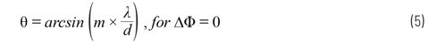
From this simplification, it is evident that if λ/d is >1, then only m = 0 could give an argument that is bounded between –1 and +1. And that argument will just be 0, and the arcsin(0) = 0°, the mechanical boresight angle. So, this is all as we would expect. Furthermore, for any m ≥1, the arcsin argument will be too large (>1) and the resulting answer will not be real. We will see no grating lobes for θ = 0 and d <λ!

However, if d >λ (therefore λ/d is <1), then multiple solutions, grating lobes, could exist. For example, if λ/d = 0.66 (that is, d = 1.5λ), then real arcsin solutions would exist for m = 0 and for m = ±1. That m = ±1 is the second solution, which is the spatial aliasing of the desired signal. Therefore, we can expect to see three main lobes, each with approximately equal amplitude, located at arcsin(0 × 0.66), arcsin(1 × 0.66), and arcsin(–1 × 0.66). In degrees, these angles are 0° and ±41.3°. In fact, this is what our array factor plot shows in Figure 3.

Figure 3. Array factor at boresight for d/λ = 1.5, N = 8.

Grating Lobes for λ/2 <d <λ

In simplifying the grating lobe equation (Equation 5), we chose to only look at mechanical boresight (∆Φ = 0). And we saw that, at mechanical boresight, grating lobes would not appear for d <λ. But from our analogy of sampling theory, we know that we should also expect to see some kind of grating lobe for any spacing greater than λ/2. So where are the grating lobes for λ/2 <d <λ?

First, recall how the phase changed with steering angle in Figure 4 from Part 1. We saw ∆Φ range from 0 to ±π as the main lobe deviated from mechanical boresight. Therefore,

will range

And for |m| ≥1, it will always be something beyond

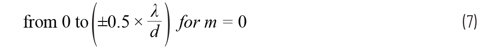
This restricts the minimum permissible λ/d if we want to keep the entire arcsin argument >1 for all |m| ≥1. Consider two cases:

• If λ/d ≥2 (that is, d ≤λ/2), then you could never have multiple solutions, regardless of the value of m. All m >0 solutions will result in an arcsin argument >1. This is the only way to avoid grating lobes to the horizon.
• But if we purposefully restricted ∆Φ to something less than ±π, then we could tolerate a smaller λ/d and still not see grating lobes. Reducing the rangeof ∆Φ means reducing the maximum steering angle of our array. It is an interesting trade-off that will be explored in the next section.

Element Spacing Considerations

Should the element spacing always be less than λ/2? Not necessarily! This becomes a trade-off for the antenna designer to consider. If the beam is steered completely to the horizon, then θ = ±90°, and an element spacing of λ/2 is required (if no grating lobes are allowed in the visiblehemisphere). But in practice, the maximum achievable steering angle is always less than 90°. This is due to the element factor and other degradations at large steering angles.

From the arcsin figure, Figure 2, we can see that if the y axis, θ, is restricted to a reduced limit, then grating lobes only occur at scan angles that are not used anyway. What would this reduced limit (θmax) be for a given element spacing (dmax)? We had said previously that our goal is to keep

We can use this to calculate where our first grating lobe (m = ±1) would appear. Making this change, and using Equation 1 from Part 1 for ∆Φ, gives:

Which simplifies to

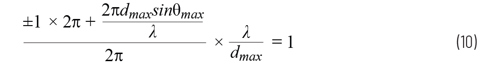
Then solving for dmax

This dmax is the condition for no grating lobes in the reduced scan angle (θmax), where θmax is less than π/2 (90°). For example, if the signal frequency is10GHz and we need to steer ±50° without grating lobes, then the maximum element spacing is:

Figure 4. Grating lobes starting to appear at the horizon for θ = 50°, N = 32, d = 17mm, and Φ = 10GHz.

Restricting the maximum scan angle, then, brings a freedom to extend the element spacing to increase the physical size per channel and to extend the aperture for a given number of elements. An example application that could exploit this phenomenon is for an antenna assigned to a fairly narrow predefined direction. The element gain can be increased for directivity in the predefined direction and the element spacing can also be increased for a larger aperture. Both result in larger overall antenna gain within the narrowed beam angle.

Note that Equation 3 indicates a maximum spacing of one wavelength, even for zero steering angle. This is the case if grating lobes cannot be tolerated in the visible hemisphere. In the case of a GEO satellite, for example, the entire Earth is covered with a steering angle of 9° from mechanical boresight. It may be the case that grating lobes can be tolerated, as long as they don’t land on the Earth’s surface. In such a case, the element spacing can be several wavelengths, resulting in even more narrow beamwidths.

There are also antenna architectures worth noting that attempt to overcome the grating lobe problem by producing a non-uniform element spacing. These are categorised as aperiodic arrays, with spiral arrays as an example. For mechanical antenna construction reasons, it may be desirable to have a common building block that can be scaled to a larger array, but this would produce a uniform array that is subject to the grating lobe conditions described.

Beam Squint

We opened Part 1 by describing how, when a wavefront approaches an array of elements, there is a time delay between elements based on the wavefront angle θ relative to boresight. For a single frequency, the beam steering can be accomplished by replacing the time delay with a phase shift. This works for narrow-band waveforms, but for wideband waveforms where the beam steering is produced by a phase shift, the beam can shift direction as a function of frequency. This can be intuitively explained if we remember that a time delay is a linear phase shift vs. frequency. Thus, for a given beam direction, the phase shift required changes as a function of frequency. Or conversely for a given phase shift, the beam directionchanges as a function of frequency. The concept of the beam angle changing as a function of frequency is called beam squint.

Figure 5. Beam squint example at X-band for a 32-element linear array with a λ/2 element spacing.

Also consider that at boresight, θ = 0, there is no phase shift across the elements and therefore no means to produce any beam squint. Therefore, the amount of beam squint must be a function of angle, θ, as well as the frequency variation. Figure 5 shows an X-band example. In this example, thecentre frequency is 10GHz, the modulation bandwidth is 2GHz, and it is apparent that the beam changes direction as a function of both frequency andthe initial beam angle.

Beam squint can be calculated directly. Using Equation 1 and Equation 2, the beam direction deviation, beam squint, can be calculated as

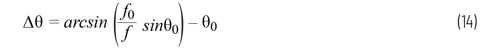
This equation is shown graphically in Figure 6. In Figure 6, the f/f0 ratio shown is intentional. The reciprocal of (f0/f) from the previous equationprovides an easier way to visualise the change relative to a centre frequency.

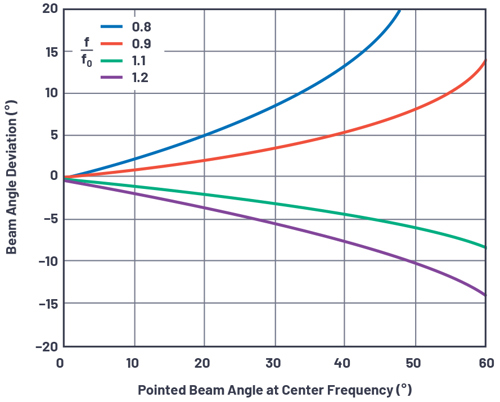Figure 6. Beam squint vs. beam angle for several frequency deviations.

A few observations on beam squint:

• The deviation in beam angle vs. frequency increases as beam angle away from boresight increases.
• A frequency below the centre frequency causes a larger deviation than a frequency above the centre frequency.
• A frequency below the centre frequency moves the beam further away from boresight.

Beam Squint Considerations

The beam squint, deviation in steering angle vs. frequency, is caused by approximating a time delay with a phase shift. Implementing beam steering with true time delay units does not have this problem.

With the beam squint problem so clearly visible, why would anyone use a phase shifter over a time delay unit? Typically, this comes down to design simplicity and IC availability of phase shifters vs. time delays. Time delays are implemented in some form of transmission line and the total delayneeded is a function of the aperture size. To date, most available analogue beamforming ICs are phase shift based, but there are families of true time delay ICs emerging and these may become much more common for phased array implementations.

In digital beamforming, true time delay can be implemented in the DSP logic and digital beamforming algorithms. Therefore, a phased array architecture where every element is digitised would lend itself naturally to overcome the beam squint problem, while also providing the mostprogrammable flexibility. However, the power, size, and cost of such a solution can be problematic.

In hybrid beamforming, there is a combination of analogue beamforming for sub-arrays followed by digital beamforming for the full array. This canoffer some natural beam squint mitigation worth considering. Beam squint is only subject to the sub-array, which is a much wider beamwidth, so it ismore tolerant to a beam angle deviation. Thus, as long as the sub-array beam squint is tolerable, then the hybrid beamforming architecture can beimplemented with phase shifters in the sub-arrays followed by true time delay in the digital beamforming.

Summary

This concludes Part 2 of a three-part series on phased array antenna patterns. In Part 1, we introduced beam pointing and the array factor. In Part 2,we introduced imperfections of grating lobes and beam squint. In Part 3, we will discuss tapering as a method to reduce sidelobes, and also provideinsight into the impact of phase shifter quantisation errors.

 
Analog Devices: www.analog.com

 
References
Balanis, Constantine A. Antenna Theory: Analysis and Design, third edition. Wiley-Interscience, 2005.

Longbrake, Matthew. True Time Delay Beamsteering for Radar. 2012 IEEE National Aerospace and Electronics Conference (NAECON), IEEE, 2012.

Mailloux, Robert J. Phased Array Antenna Handbook, second edition. Artech House, 2005.

O’Donnell, Robert M. “Radar Systems Engineering: Introduction.” IEEE, June 2012.

Skolnik, Merrill. Radar Handbook, third edition. McGraw Hill, 2008.

About the Author
Peter Delos is a technical lead in the Aerospace and Defense Group at Analog Devices in Greensboro, NC. He received his B.S.E.E. from Virginia Tech in 1990 and M.S.E.E. from NJIT in 2004. Peter has over 25 years of industry experience. Most of his career has been spent designing advanced RF/analogue systems at the architecture level, PWB level, and IC level. He is currently focused on miniaturising high performance receiver, waveform generator, and synthesiser designs for phased array applications. He can be reached at peter.delos@analog.com.

About the Author
Bob Broughton started at Analog Devices in 1993 and has held positions as a product engineer and an IC design engineer, and is currently the director of engineering in the Aerospace and Defense Business Unit. Prior to ADI, Bob worked at Raytheon as an RF design engineer and at Peregrine Semiconductor as an RFIC designer. Bob graduated with a B.S.E.E. from West Virginia University in 1984. He can be reached at bob.broughton@analog.com.

About the Author
Jon Kraft is a senior staff FAE in Colorado and has been with ADI for 13 years. His focus is software-defined radio and aerospace phased array radar. He received his B.S.E.E. from Rose-Hulman and his M.S.E.E. from Arizona State University. He has nine patents issued, six with ADI, and one currently pending. He can be reached at jon.kraft@analog.com.